Higher-dimensional Interpolation
Higher-dimensional Interpolation Contents
Two-dimensional interpolation
There are two types of two-dimensional interpolation classes, the first is based on a function defined on a two-dimensional grid (though the spacings between grid points need not be equal). The class interp2_direct implements bilinear or bicubic interpolation, and is based on D. Zaslavsky’s routines at https://github.com/diazona/interp2d (licensed under GPLv3). A slightly slower (but a bit more flexible) alternative is successive use of interp_base objects, implemented in interp2_seq .
If data is arranged without a grid, then interp2_neigh performs nearest-neighbor interpolation. At present, the only way to compute contour lines on data which is not defined on a grid is to use this class or one of the multi-dimensional interpolation classes described below the data on a grid and then use contour afterwards.
Multi-dimensional interpolation
Multi-dimensional interpolation for table defined on a grid is
possible with tensor_grid. See the documentation
for o2scl::tensor_grid::interpolate(),
o2scl::tensor_grid::interp_linear() and
o2scl::tensor_grid::rearrange_and_copy(). Also, if you
want to interpolate rank-1 indices to get a vector result, you can
use o2scl::tensor_grid::interp_linear_vec() .
If the data is not on a grid, then inverse distance weighted interpolation is performed by interpm_idw.
An experimental class for multidimensional-dimensional kriging is also provided in interpm_krige_optim .
Finally, an experimental Python interface for interpolation using either Gaussian processes or neural networks from O₂sclpy is provided in interpm_python when Python support is enabled.
Interpolation on a rectangular grid
This example creates a sample 3 by 3 grid of data with the function \(\left[ \sin \left( x/10 + 3 y/10 \right) \right]^2\) and performs some interpolations and compares them with the exact result.
Data:
          x  | 0.000000e+00 1.000000e+00 2.000000e+00
 y           |
-------------|----------------------------------------
3.000000e+00 | 6.136010e-01 7.080734e-01 7.942506e-01
2.000000e+00 | 3.188211e-01 4.150164e-01 5.145998e-01
1.000000e+00 | 8.733219e-02 1.516466e-01 2.298488e-01

x            y            Calc.        Exact
5.000000e-01 1.500000e+00 6.070521e-01 2.298488e-01
9.900000e-01 1.990000e+00 4.187808e-01 4.110774e-01
1.000000e+00 2.000000e+00 4.150164e-01 4.150164e-01

5.000000e-01 1.500000e+00 6.070521e-01 2.298488e-01
9.900000e-01 1.990000e+00 4.187808e-01 4.110774e-01
1.000000e+00 2.000000e+00 4.150164e-01 4.150164e-01

0 tests performed.
All tests passed.
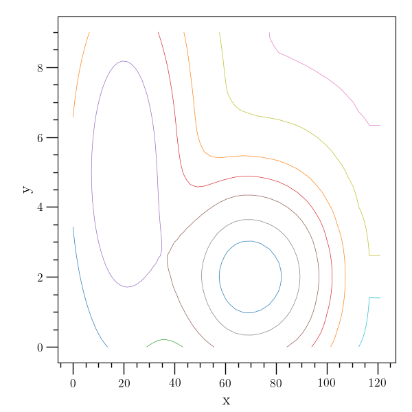
Contour lines
This example generates contour lines of the function
The figure below shows contour lines in the region \(x\in(0,121), y\in(0,9)\). The data grid is represented by plus signs, and the associated generated contours. The figure clearly shows the peaks at \((20,5)\) and \((70,2)\).

The contour class can also use interpolation to attempt to refine the data grid. The new contours after a refinement of a factor of 5 is given in the figure below.