Ordinary Differential Equations
Ordinary differential equations contents
Ordinary differential equations introduction
Classes for non-adaptive integration are provided as descendents of ode_step and classes for adaptive integration are descendants of astep_base. To specify a set of functions to these classes, use a child of ode_funct for a generic vector type. The classes ode_rkf45_gsl and ode_rkck_gsl are reasonable general-purpose non-adaptive integrators and astep_gsl is a good general-purpose adaptive method for non-stiff problems. For stiff ODE’s, use ode_bsimp_gsl (see Stiff differential equations example).
Solution of simple initial value problems is performed by ode_iv_solve. This class uses an adaptive integrator (default is astep_gsl) and does some bookkeeping to simplify the solution of initial value problems. The ode_iv_solve class will give the final value of the functions at the endpoint, provide the functions on a user-specified grid, or it will tabulate the ODE solution for you using the grid chosen with the adaptive stepper. A example demonstrating the solution of initial value problems is given in the Ordinary differential equations example.
The solution of boundary-value problems is based on the abstract base class ode_bv_solve. At the moment, a simple shooting method is the only implementation of this base class and is given in ode_bv_shoot . An experimental multishooting class is given in ode_bv_mshoot.
An application of linear solvers to solve finite-difference equations approximating a boundary value problem is given in ode_it_solve. A example demonstrating the iterative solution of a boundary value problem is given in the Iterative solution of ODEs example.
Ordinary differential equations example
This example solves the differential equations defining the the Bessel and Airy functions with both the Cash-Karp and Prince-Dormand steppers. It demonstrates the use of ode_rkck_gsl, ode_rk8pd_gsl, astep_gsl, and ode_iv_solve and stores the results in table objects.
The Bessel functions are defined by
The Bessel functions of the first kind, \(J_{\alpha}(x)\) are finite at the origin, and the example solves the \(\alpha=1\) case, where \(J_1(0) = 0\) and \(J_1^{\prime}(0) = 1/2\).
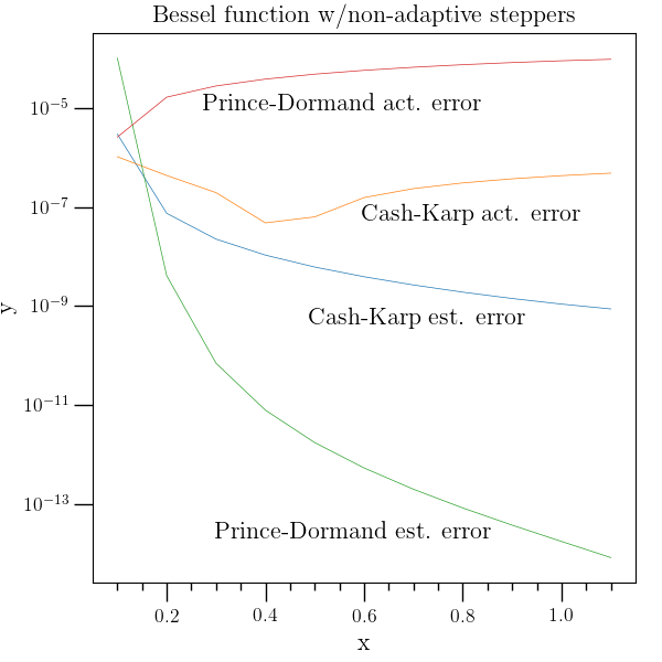
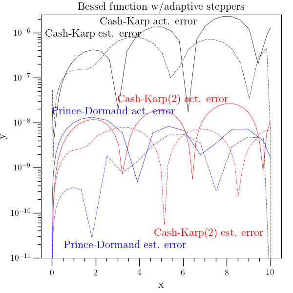
Note that with a Bessel function and a fixed step size, the Prince-Dormand stepper (even though of higher order than the Cash-Karp stepper) is actually less accurate, and seriously underestimates the error.
The Airy functions are defined by
This example solves for the Airy function of the first kind, \(Ai(x)\).
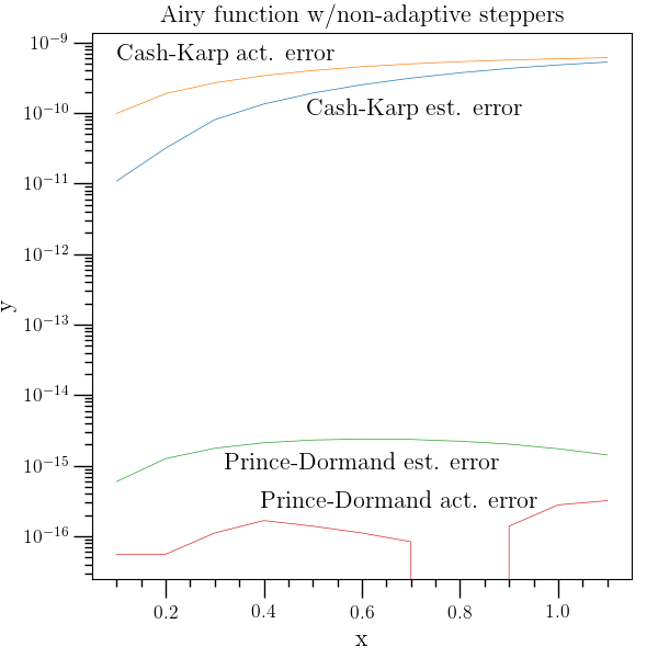
Here the higher order stepper is more accurate.
Ordinary differential equations example source code
/* Example: ex_ode.cpp
   -------------------------------------------------------------------
   An example to demonstrate solving differential equations. See "License
   Information" section of the documentation for license information.
*/

#include <boost/numeric/ublas/vector.hpp>
#include <boost/numeric/ublas/matrix.hpp>
#include <boost/numeric/ublas/matrix_proxy.hpp>
#include <gsl/gsl_sf_bessel.h>
#include <gsl/gsl_sf_airy.h>
#include <gsl/gsl_sf_gamma.h>
#include <o2scl/test_mgr.h>
#include <o2scl/ode_funct.h>
#include <o2scl/ode_rkck_gsl.h>
#include <o2scl/ode_rk8pd_gsl.h>
#include <o2scl/astep_gsl.h>
#include <o2scl/ode_iv_solve.h>
#include <o2scl/table.h>
#include <o2scl/hdf_file.h>
#include <o2scl/hdf_io.h>

using namespace std;
using namespace o2scl;
using namespace o2scl_hdf;

typedef boost::numeric::ublas::vector<double> ubvector;
typedef boost::numeric::ublas::matrix<double> ubmatrix;
typedef boost::numeric::ublas::matrix_row<ubmatrix> ubmatrix_row;

// Differential equation defining the Bessel function. This assumes
// the second derivative at x=0 is 0 and thus only works for odd alpha.
int derivs(double x, size_t nv, const ubvector &y,
	   ubvector &dydx, double &alpha) {
  dydx[0]=y[1];
  if (x==0.0) dydx[1]=0.0;
  else dydx[1]=(-x*y[1]+(-x*x+alpha*alpha)*y[0])/x/x;
  return 0;
}

// Differential equation defining the Airy function, Ai(x)
int derivs2(double x, size_t nv, const ubvector &y,
	    ubvector &dydx) {
  dydx[0]=y[1];
  dydx[1]=y[0]*x;
  return 0;
}

// Differential equation defining the Bessel function using
// a vector object for o2scl::ode_iv_solve_grid
int derivs3(double x, size_t nv, const o2scl::solve_grid_mat_row &y,
	    o2scl::solve_grid_mat_row &dydx, double &alpha) {
  dydx[0]=y[1];
  if (x==0.0) dydx[1]=0.0;
  else dydx[1]=(-x*y[1]+(-x*x+alpha*alpha)*y[0])/x/x;
  return 0;
}

int main(void) {

  cout.setf(ios::scientific);
  cout.setf(ios::showpos);

  // The independent variable and stepsize
  double x, dx=1.0e-1;

  // The function and derivative values and the estimated errors
  ubvector y(2), dydx(2), yout(2), yerr(2), dydx_out(2);

  test_mgr t;
  t.set_output_level(1);

  // The parameter for the Bessel function
  double alpha=1.0;

  // Specify the differential equations to solve
  ode_funct od=
    std::bind(derivs,std::placeholders::_1,std::placeholders::_2,
	      std::placeholders::_3,std::placeholders::_4,alpha);
  ode_funct od2=derivs2;
  ode_funct_solve_grid od3=
    std::bind(derivs3,std::placeholders::_1,std::placeholders::_2,
	      std::placeholders::_3,std::placeholders::_4,alpha);

  // The basic ODE steppers
  ode_rkck_gsl<> ode;
  ode_rk8pd_gsl<> ode2;

  // ------------------------------------------------------------
  // Store the results in tables

  table<> tab[8];
  tab[0].line_of_names("x calc exact diff err");
  tab[1].line_of_names("x calc exact diff err");
  tab[2].line_of_names("x calc exact diff err");
  tab[3].line_of_names("x calc exact diff err");
  tab[4].line_of_names("x calc exact diff err0 err1");
  tab[5].line_of_names("x calc exact diff err0 err1");
  tab[6].line_of_names("x calc exact diff err0 err1");
  tab[7].line_of_names("x calc exact diff err0");

  // ------------------------------------------------------------
  // Solution 1: Solve using the non-adaptive Cash-Karp stepper.

  cout << "Bessel function, Cash-Karp: " << endl;

  // Initial values at x=0
  x=0.0;
  y[0]=0.0;
  y[1]=0.5;

  // The non-adaptive ODE steppers require the derivatives as
  // input
  derivs(x,2,y,dydx,alpha);

  cout << " x             J1(calc)      J1(exact)     rel. diff.    "
       << "err" << endl;

  while (x<1.0) {

    // Perform a step. Since the fourth and sixth arguments are
    // the same, the values in 'y' are updated with the new values
    // at x+dx.
    ode.step(x,dx,2,y,dydx,y,yerr,dydx,od);

    // Update the x value
    x+=dx;

    // Print and test
    cout << x << " " << y[0] << " "
	 << gsl_sf_bessel_J1(x) << " ";
    cout << fabs((y[0]-gsl_sf_bessel_J1(x))/gsl_sf_bessel_J1(x)) << " ";
    cout << yerr[0] << endl;
    t.test_rel(y[0],gsl_sf_bessel_J1(x),5.0e-5,"rkck");

    // Also output the results to a table
    vector<double> line={x,y[0],gsl_sf_bessel_J1(x),
      fabs((y[0]-gsl_sf_bessel_J1(x))/gsl_sf_bessel_J1(x)),
      yerr[0]};
    tab[0].line_of_data(line.size(),line);
  }

  // Compare with the exact result at the last point
  cout << "Accuracy at end: "
       << fabs(y[0]-gsl_sf_bessel_J1(x))/gsl_sf_bessel_J1(x) << endl;
  cout << endl;

  // End of Solution 1
  // ------------------------------------------------------------
  // Solution 2: Solve using the non-adaptive Prince-Dormand stepper.
  // Note that for the Bessel function, the 8th order stepper performs
  // worse than the 4th order. The error returned by the stepper is
  // larger near x=0, as expected.

  cout << "Bessel function, Prince-Dormand: " << endl;
  x=0.0;
  y[0]=0.0;
  y[1]=0.5;
  derivs(x,2,y,dydx,alpha);
  cout << " x             J1(calc)      J1(exact)     rel. diff.    "
       << "err" << endl;
  while (x<1.0) {
    ode2.step(x,dx,2,y,dydx,y,yerr,dydx,od);
    x+=dx;
    cout << x << " " << y[0] << " "
	 << gsl_sf_bessel_J1(x) << " ";
    cout << fabs((y[0]-gsl_sf_bessel_J1(x))/gsl_sf_bessel_J1(x)) << " ";
    cout << yerr[0] << endl;
    t.test_rel(y[0],gsl_sf_bessel_J1(x),5.0e-4,"rk8pd");

    // Also output the results to a table
    vector<double> line={x,y[0],gsl_sf_bessel_J1(x),
      fabs((y[0]-gsl_sf_bessel_J1(x))/gsl_sf_bessel_J1(x)),
      yerr[0]};
    tab[1].line_of_data(line.size(),line);
  }
  cout << "Accuracy at end: "
       << fabs(y[0]-gsl_sf_bessel_J1(x))/gsl_sf_bessel_J1(x) << endl;
  cout << endl;

  // End of Solution 2
  // ------------------------------------------------------------
  // Solution 3: Solve using the non-adaptive Cash-Karp stepper.

  cout << "Airy function, Cash-Karp: " << endl;
  x=0.0;
  y[0]=1.0/pow(3.0,2.0/3.0)/gsl_sf_gamma(2.0/3.0);
  y[1]=-1.0/pow(3.0,1.0/3.0)/gsl_sf_gamma(1.0/3.0);
  derivs2(x,2,y,dydx);
  cout << " x             Ai(calc)      Ai(exact)     rel. diff.    "
       << "err" << endl;
  while (x<1.0) {
    ode.step(x,dx,2,y,dydx,y,yerr,dydx,od2);
    x+=dx;
    cout << x << " " << y[0] << " "
	 << gsl_sf_airy_Ai(x,GSL_PREC_DOUBLE) << " ";
    cout << fabs((y[0]-gsl_sf_airy_Ai(x,GSL_PREC_DOUBLE))/
		 gsl_sf_airy_Ai(x,GSL_PREC_DOUBLE)) << " ";
    cout << yerr[0] << endl;
    t.test_rel(y[0],gsl_sf_airy_Ai(x,GSL_PREC_DOUBLE),1.0e-8,"rkck");

    // Also output the results to a table
    vector<double> line={x,y[0],gsl_sf_airy_Ai(x,GSL_PREC_DOUBLE),
      fabs((y[0]-gsl_sf_airy_Ai(x,GSL_PREC_DOUBLE))/
           gsl_sf_airy_Ai(x,GSL_PREC_DOUBLE)),
      yerr[0]};
    tab[2].line_of_data(line.size(),line);
  }
  cout << "Accuracy at end: "
       << fabs(y[0]-gsl_sf_airy_Ai(x,GSL_PREC_DOUBLE))/
    gsl_sf_airy_Ai(x,GSL_PREC_DOUBLE) << endl;
  cout << endl;

  // End of Solution 3
  // ------------------------------------------------------------
  // Solution 4: Solve using the non-adaptive Prince-Dormand stepper.
  // On this function, the higher-order routine performs significantly
  // better.

  cout << "Airy function, Prince-Dormand: " << endl;
  x=0.0;
  y[0]=1.0/pow(3.0,2.0/3.0)/gsl_sf_gamma(2.0/3.0);
  y[1]=-1.0/pow(3.0,1.0/3.0)/gsl_sf_gamma(1.0/3.0);
  derivs2(x,2,y,dydx);
  cout << " x             Ai(calc)      Ai(exact)     rel. diff.    "
       << "err" << endl;
  while (x<1.0) {
    ode2.step(x,dx,2,y,dydx,y,yerr,dydx,od2);
    x+=dx;
    cout << x << " " << y[0] << " "
	 << gsl_sf_airy_Ai(x,GSL_PREC_DOUBLE) << " ";
    cout << fabs((y[0]-gsl_sf_airy_Ai(x,GSL_PREC_DOUBLE))/
		 gsl_sf_airy_Ai(x,GSL_PREC_DOUBLE)) << " ";
    cout << yerr[0] << endl;
    t.test_rel(y[0],gsl_sf_airy_Ai(x,GSL_PREC_DOUBLE),1.0e-14,"rk8pd");

    // Also output the results to a table
    vector<double> line={x,y[0],gsl_sf_airy_Ai(x,GSL_PREC_DOUBLE),
      fabs((y[0]-gsl_sf_airy_Ai(x,GSL_PREC_DOUBLE))/
           gsl_sf_airy_Ai(x,GSL_PREC_DOUBLE)),
      yerr[0]};
    tab[3].line_of_data(line.size(),line);
  }
  cout << "Accuracy at end: "
       << fabs(y[0]-gsl_sf_airy_Ai(x,GSL_PREC_DOUBLE))/
    gsl_sf_airy_Ai(x,GSL_PREC_DOUBLE) << endl;
  cout << endl;

  // End of Solution 4
  // ------------------------------------------------------------
  // Solution 5: Solve using the GSL adaptive stepper

  // Lower the output precision to fit in 80 columns
  cout.precision(5);

  cout << "Adaptive stepper: " << endl;
  astep_gsl<> ode3;
  x=0.0;
  y[0]=0.0;
  y[1]=0.5;
  cout << "   x            J1(calc)     J1(exact)    rel. diff.";
  cout << "   err_0        err_1" << endl;
  int k=0;
  while (x<10.0) {
    int retx=ode3.astep(x,10.0,dx,2,y,dydx,yerr,od);
    if (k%3==0) {
      cout << retx << " " << x << " " << y[0] << " "
	   << gsl_sf_bessel_J1(x) << " ";
      cout << fabs((y[0]-gsl_sf_bessel_J1(x))/gsl_sf_bessel_J1(x)) << " ";
      cout << yerr[0] << " " << yerr[1] << endl;
    }
    t.test_rel(y[0],gsl_sf_bessel_J1(x),5.0e-3,"astep");
    t.test_rel(y[1],0.5*(gsl_sf_bessel_J0(x)-gsl_sf_bessel_Jn(2,x)),
               5.0e-3,"astep 2");
    t.test_rel(yerr[0],0.0,4.0e-6,"astep 3");
    t.test_rel(yerr[1],0.0,4.0e-6,"astep 4");
    t.test_gen(retx==0,"astep 5");

    // Also output the results to a table
    vector<double> line={x,y[0],gsl_sf_bessel_J1(x),
      fabs((y[0]-gsl_sf_bessel_J1(x))/gsl_sf_bessel_J1(x)),
      yerr[0],yerr[1]};
    tab[4].line_of_data(line.size(),line);

    k++;
  }
  cout << "Accuracy at end: "
       << fabs(y[0]-gsl_sf_bessel_J1(x))/gsl_sf_bessel_J1(x) << endl;
  cout << endl;

  // End of Solution 5
  // ------------------------------------------------------------
  // Solution 6: Solve using the GSL adaptive stepper.
  // Decrease the tolerances, and the adaptive stepper takes
  // smaller step sizes.

  cout << "Adaptive stepper with smaller tolerances: " << endl;
  ode3.con.eps_abs=1.0e-8;
  ode3.con.a_dydt=1.0;
  x=0.0;
  y[0]=0.0;
  y[1]=0.5;
  cout << "   x            J1(calc)     J1(exact)    rel. diff.";
  cout << "   err_0        err_1" << endl;
  k=0;
  while (x<10.0) {
    int retx=ode3.astep(x,10.0,dx,2,y,dydx,yerr,od);
    if (k%3==0) {
      cout << retx << " " << x << " " << y[0] << " "
	   << gsl_sf_bessel_J1(x) << " ";
      cout << fabs((y[0]-gsl_sf_bessel_J1(x))/gsl_sf_bessel_J1(x)) << " ";
      cout << yerr[0] << " " << yerr[1] << endl;
    }
    t.test_rel(y[0],gsl_sf_bessel_J1(x),5.0e-3,"astep");
    t.test_rel(y[1],0.5*(gsl_sf_bessel_J0(x)-gsl_sf_bessel_Jn(2,x)),
               5.0e-3,"astep 2");
    t.test_rel(yerr[0],0.0,4.0e-8,"astep 3");
    t.test_rel(yerr[1],0.0,4.0e-8,"astep 4");
    t.test_gen(retx==0,"astep 5");

    // Also output the results to a table
    vector<double> line={x,y[0],gsl_sf_bessel_J1(x),
      fabs((y[0]-gsl_sf_bessel_J1(x))/gsl_sf_bessel_J1(x)),
      yerr[0],yerr[1]};
    tab[5].line_of_data(line.size(),line);

    k++;
  }
  cout << "Accuracy at end: "
       << fabs(y[0]-gsl_sf_bessel_J1(x))/gsl_sf_bessel_J1(x) << endl;
  cout << endl;

  // End of Solution 6
  // ------------------------------------------------------------
  // Solution 7: Solve using the GSL adaptive stepper.
  // Use the higher-order stepper, and less steps are required. The
  // stepper automatically takes more steps near x=0 in order since
  // the higher-order routine has more trouble there.

  cout << "Adaptive stepper, Prince-Dormand: " << endl;
  ode3.set_step(ode2);
  x=0.0;
  y[0]=0.0;
  y[1]=0.5;
  cout << "   x            J1(calc)     J1(exact)    rel. diff.";
  cout << "   err_0        err_1" << endl;
  k=0;
  while (x<10.0) {
    int retx=ode3.astep(x,10.0,dx,2,y,dydx,yerr,od);
    if (k%3==0) {
      cout << retx << " " << x << " " << y[0] << " "
	   << gsl_sf_bessel_J1(x) << " ";
      cout << fabs((y[0]-gsl_sf_bessel_J1(x))/gsl_sf_bessel_J1(x)) << " ";
      cout << yerr[0] << " " << yerr[1] << endl;
    }
    t.test_rel(y[0],gsl_sf_bessel_J1(x),5.0e-3,"astep");
    t.test_rel(y[1],0.5*(gsl_sf_bessel_J0(x)-gsl_sf_bessel_Jn(2,x)),
               5.0e-3,"astep");
    t.test_rel(yerr[0],0.0,4.0e-8,"astep 3");
    t.test_rel(yerr[1],0.0,4.0e-8,"astep 4");
    t.test_gen(retx==0,"astep 5");

    // Also output the results to a table
    vector<double> line={x,y[0],gsl_sf_bessel_J1(x),
      fabs((y[0]-gsl_sf_bessel_J1(x))/gsl_sf_bessel_J1(x)),
      yerr[0],yerr[1]};
    tab[6].line_of_data(line.size(),line);

    k++;
  }
  cout << "Accuracy at end: "
       << fabs(y[0]-gsl_sf_bessel_J1(x))/gsl_sf_bessel_J1(x) << endl;
  cout << endl;

  // End of Solution 7
  // ------------------------------------------------------------
  // Solution 8: Solve using the O2scl initial value solver

  // Return the output precision to the default
  cout.precision(6);

  cout << "Initial value solver: " << endl;
  ode_iv_solve_grid<> ode4;
  ode4.ntrial=10000;

  // Define the grid and the storage for the solution
  const size_t ngrid=101;
  ubvector xg(ngrid), yinit(2);
  ubmatrix yg(ngrid,2), ypg(ngrid,2), yerrg(ngrid,2);
  for(size_t i=0;i<ngrid;i++) xg[i]=((double)i)/10.0;

  // Set the initial value
  xg[0]=0.0;
  xg[ngrid-1]=10.0;
  yg(0,0)=0.0;
  yg(0,1)=0.5;

  // Perform the full solution
  ode4.solve_grid<ubvector,ubmatrix>(0.1,2,ngrid,xg,yg,yerrg,ypg,od3);

  // Output and test the results
  cout << " x             J1(calc)      J1(exact)     rel. diff." << endl;
  for(size_t i=1;i<ngrid;i++) {

    if (i%10==0) {
      cout << xg[i] << " " << yg(i,0) << " "
	   << gsl_sf_bessel_J1(xg[i]) << " ";
      cout << fabs(yg(i,0)-gsl_sf_bessel_J1(xg[i])) << " "
	   << fabs(yerrg(i,0)) << endl;
    }
    t.test_rel(yg(i,0),gsl_sf_bessel_J1(xg[i]),5.0e-7,"astep");
    t.test_rel(yg(i,1),0.5*(gsl_sf_bessel_J0(xg[i])-
                             gsl_sf_bessel_Jn(2,xg[i])),5.0e-7,"astep 2");

    // Also output the results to a table
    vector<double> line={xg[i],yg(i,0),gsl_sf_bessel_J1(xg[i]),
      fabs(yg(i,0)-gsl_sf_bessel_J1(xg[i])),
      fabs(yerrg(i,0))};
    tab[7].line_of_data(line.size(),line);
  }

  cout << "Accuracy at end: "
       << fabs(yg(ngrid-1,0)-gsl_sf_bessel_J1(xg[ngrid-1]))/
    gsl_sf_bessel_J1(xg[ngrid-1]) << endl;
  cout << endl;

  // End of Solution 8
  // ------------------------------------------------------------
  // Output results to a file

  hdf_file hf;
  hf.open_or_create("ex_ode.o2");
  for(size_t i=0;i<8;i++) {
    hdf_output(hf,tab[i],((string)"table_")+itos(i));
  }
  hf.close();

  // ------------------------------------------------------------

  cout.unsetf(ios::showpos);
  t.report();

  return 0;
}
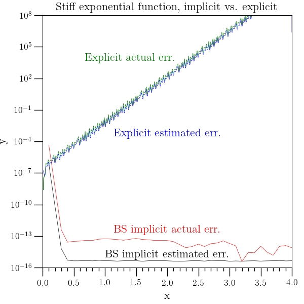
Stiff differential equations example
This example solves the differential equations
which have the exact solution
using both the stiff stepper ode_bsimp_gsl and the standard adaptive stepper astep_gsl . The relative error on the adaptive stepper is orders of magnitude larger.
/* Example: ex_stiff.cpp
   -------------------------------------------------------------------
   An example to demonstrate solving stiff differential equations
*/

#include <boost/numeric/ublas/vector.hpp>
#include <boost/numeric/ublas/matrix.hpp>

#include <o2scl/test_mgr.h>
#include <o2scl/funct.h>
#include <o2scl/ode_funct.h>
#include <o2scl/astep_gsl.h>
#include <o2scl/ode_bsimp_gsl.h>
#include <o2scl/table.h>

#ifdef O2SCL_HDF
#include <o2scl/hdf_file.h>
#include <o2scl/hdf_io.h>
#endif

using namespace std;
using namespace o2scl;
#ifdef O2SCL_HDF
using namespace o2scl_hdf;
#endif

typedef boost::numeric::ublas::vector<double> ubvector;
typedef boost::numeric::ublas::matrix<double> ubmatrix;

int derivs(double x, size_t nv, const ubvector &y,
	   ubvector &dydx) {
  dydx[0]=480.0*y[0]+980.0*y[1];
  dydx[1]=-490.0*y[0]-990.0*y[1];
  return 0;
}

int jac(double x, size_t nv, const ubvector &y,
	ubmatrix &dfdy, ubvector &dfdx) {
  dfdy(0,0)=480.0;
  dfdy(0,1)=980.0;
  dfdy(1,0)=-490.0;
  dfdy(1,1)=-990.0;
  dfdx[0]=0.0;
  dfdx[1]=0.0;
  return 0;
}

int main(void) {
  test_mgr t;
  t.set_output_level(1);

  cout.setf(ios::scientific);
  cout.precision(3);

  // Specification of the differential equations and the Jacobian
  ode_funct od11=derivs;
  ode_jac_funct oj=jac;

  table<> tab[2];
  tab[0].line_of_names("x calc exact rel_err rel_diff");
  tab[1].line_of_names("x calc exact rel_err rel_diff");

  // ------------------------------------------------------------
  // First solve with ode_bsimp_gsl, designed to handle stiff ODEs

  ode_bsimp_gsl<> gb;

  double x1, dx=1.0e-1;
  ubvector y1(2), dydx1(2), yout1(2), yerr1(2), dydx_out1(2);

  x1=0.0;
  y1[0]=1.0;
  y1[1]=0.0;

  derivs(x1,2,y1,dydx1);

  for(size_t i=1;i<=40;i++) {

    gb.step(x1,dx,2,y1,dydx1,y1,yerr1,dydx1,od11,oj);
    x1+=dx;

    double exact[2]={-exp(-500.0*x1)+2.0*exp(-10.0*x1),
		     exp(-500.0*x1)-exp(-10.0*x1)};

    cout.setf(ios::showpos);
    cout << x1 << " " << y1[0] << " " << y1[1] << " "
	 << yerr1[0] << " " << yerr1[1] << " " << exact[0] << " "
	 << exact[1] << endl;
    cout.unsetf(ios::showpos);

    double line[5]={x1,y1[0],exact[0],fabs(yerr1[0]/exact[0]),
		    fabs((y1[0]-exact[0])/exact[0])};
    tab[0].line_of_data(5,line);

    t.test_rel(y1[0],exact[0],3.0e-4,"y0");
    t.test_rel(y1[1],exact[1],3.0e-4,"y1");

  }

  cout << endl;

  // ------------------------------------------------------------
  // Now compare to the traditional adaptive stepper

  astep_gsl<> ga;

  double x2;
  ubvector y2(2), dydx2(2), yout2(2), yerr2(2), dydx_out2(2);

  x2=0.0;
  y2[0]=1.0;
  y2[1]=0.0;

  derivs(x2,2,y2,dydx2);

  size_t j=0;
  while (x2<4.0) {

    ga.astep(x2,4.0,dx,2,y2,dydx2,yerr2,od11);

    double exact[2]={-exp(-500.0*x2)+2.0*exp(-10.0*x2),
		     exp(-500.0*x2)-exp(-10.0*x2)};

    if (j%25==0) {
      cout.setf(ios::showpos);
      cout << x2 << " " << y2[0] << " " << y2[1] << " "
	   << yerr2[0] << " " << yerr2[1] << " " << exact[0] << " "
	   << exact[1] << endl;
      cout.unsetf(ios::showpos);
    }
    j++;

    double line[5]={x2,y2[0],exact[0],fabs(yerr2[0]/exact[0]),
		    fabs((y2[0]-exact[0])/exact[0])};
    tab[1].line_of_data(5,line);

  }

  cout << endl;

  // ------------------------------------------------------------
  // Output results to a file

#ifdef O2SCL_HDF
  hdf_file hf;
  hf.open_or_create("ex_stiff.o2");
  for(size_t i=0;i<2;i++) {
    hdf_output(hf,tab[i],((string)"table_")+itos(i));
  }
  hf.close();
#endif

  // ------------------------------------------------------------

  t.report();

  return 0;

}
// End of example
Iterative solution of ODEs example
This example solves the ODEs
given the boundary conditions
by linearizing the ODEs on a mesh and using an iterative method (sometimes called relaxation). The ode_it_solve class demonstrates how this works. For this simple example, the linear system is large and the matrix is very sparse, thus ode_bv_shoot would be much faster. However, there are some problems where iterative methods succeed and shooting fails.
/* Example: ex_ode_it.cpp
   -------------------------------------------------------------------
   Demonstrate the iterative method for solving ODEs
*/

#include <o2scl/ode_it_solve.h>
#include <o2scl/ode_iv_solve.h>
#include <o2scl/linear_solver.h>

using namespace std;
using namespace o2scl;
using namespace o2scl_linalg;

// The three-dimensional ODE system
class ode_system {

public:

  // The LHS boundary conditions
  double left(size_t ieq, double x, ovector_base &yleft) {
    if (ieq==0) return yleft[0]-1.0;
    return yleft[1]*yleft[1]+yleft[2]*yleft[2]-2.0;
  }

  // The RHS boundary conditions
  double right(size_t ieq, double x, ovector_base &yright) {
    return yright[1]-3.0;
  }

  // The differential equations
  double derivs(size_t ieq, double x, ovector_base &y) {
    if (ieq==1) return y[0]+y[1];
    else if (ieq==2) return y[0]+y[2];
    return y[1];
  }

  // This is the alternative specification for ode_iv_solve for
  // comparison
  int shoot_derivs(double x, size_t nv, const ovector_base &y,
		   ovector_base &dydx) {
    dydx[0]=y[1];
    dydx[1]=y[0]+y[1];
    dydx[2]=y[0]+y[2];
    return 0;
  }

};

int main(void) {

  test_mgr t;
  t.set_output_level(1);

  cout.setf(ios::scientific);

  // The ODE solver
  ode_it_solve<ode_it_funct<ovector_base>,ovector_base,
    omatrix_base,omatrix_row,ovector_base,omatrix_base> oit;

  // The class which contains the functions to solve
  ode_system os;

  // Make function objects for the derivatives and boundary conditions
  ode_it_funct_mfptr<ode_system> f_d(&os,&ode_system::derivs);
  ode_it_funct_mfptr<ode_system> f_l(&os,&ode_system::left);
  ode_it_funct_mfptr<ode_system> f_r(&os,&ode_system::right);

  // Grid size
  size_t ngrid=40;

  // Number of ODEs
  size_t neq=3;

  // Number of LHS boundary conditions
  size_t nbleft=2;

  // Create space for the solution and make an initial guess
  ovector x(ngrid);
  omatrix y(ngrid,neq);
  for(size_t i=0;i<ngrid;i++) {
    x[i]=((double)i)/((double)(ngrid-1));
    y[i][0]=1.0+x[i]+1.0;
    y[i][1]=3.0*x[i];
    y[i][2]=-0.1*x[i]-1.4;
  }

  int pa=0;

  // Workspace objects
  omatrix A(ngrid*neq,ngrid*neq);
  ovector rhs(ngrid*neq), dy(ngrid*neq);

  // Perform the solution
  oit.verbose=1;
  oit.solve(ngrid,neq,nbleft,x,y,f_d,f_l,f_r,A,rhs,dy);

  // Compare with the initial value solver ode_iv_solve
  ode_iv_solve<> ois;
  ode_funct_mfptr<ode_system> f_sd(&os,&ode_system::shoot_derivs);
  ovector ystart(neq), yend(neq);
  for(size_t i=0;i<neq;i++) ystart[i]=y[0][i];
  ois.solve_final_value(0.0,1.0,0.01,neq,ystart,yend,f_sd);

  // Test the result
  t.test_rel(y[0][0],1.0,1.0e-3,"ya");
  t.test_rel(y[ngrid-1][0],yend[0],1.0e-3,"yb");
  t.test_rel(y[0][1],0.25951,1.0e-3,"yc");
  t.test_rel(y[ngrid-1][1],yend[1],1.0e-3,"yd");
  t.test_rel(y[0][2],-1.3902,1.0e-3,"ye");
  t.test_rel(y[ngrid-1][2],yend[2],1.0e-3,"yf");

  t.report();

  return 0;
}
// End of example